
Contents
1. Introduction
The primary purpose of the UKFE ‘R’ package is to implement the regional flood frequency methods outlined by the Flood Estimation Handbook (FEH) and associated updates. However, there are numerous other functions of use to the hydrologist. This quick guide is for the core FEH functions which lead to extreme flow estimates from single site or pooling (gauged & ungauged) and a design hydrograph using ReFH. There is no assumption that readers of this guide are experienced ‘R’ users. There is an assumption that the reader is familiar with the application of the FEH method.
For more information about the functions discussed here and further functions of the package, all the functions are detailed in a pdf via the following link:
https://cran.r-project.org/web/packages/UKFE/UKFE.pdf
Details can also be viewed in the package documentation within the ‘R’ environment. If using RStudio, you can click on packages, search for UKFE and then click on it. You will then see a list of functions; each can be clicked for more details. If you’re using base ‘R’ (it’s a bit more opaque) to get help with individual functions you can type help(FunctionName) or ?FunctionName. To get a list of the function names type ls("package:UKFE"). This latter approach also works in RStudio.
Once R is open, to get access to the package it must be installed (this only needs to be done once) and then loaded. The following commands can be entered into the console to do so. Afterwards you are ready use the package
install.packages("UKFE")library(UKFE)Table 1 provides the key functions for implementing the FEH methods:

Table 1: Key UKFE functions for implementing the FEH methods
2. Getting catchment descriptors
Catchment descriptors can be brought into the ‘R’ environment by the GetCDs function for gauged sites that are suitable for pooling or QMED. For example they can be viewed by using the GetCDs function as follows (assuming your gauged reference is 39001):
GetCDs(39001)It’s useful to store them as an ‘object’ for use with other functions. In which case you can give them a name and attribute the name to the object with ‘<-‘. For example:
CDs.39001 <- GetCDs(39001)Then when you wish to view them, the object name CDs.39001 can be entered into the console.
If you wish to derive CDs for catchments that aren’t suitable for pooling or QMED, or aren’t gauged at all, you can use the CDsXML function. The file path will need to be used and for windows operating systems, the backslashes will need to be changed to forward slashes. For example, importing some descriptors downloaded from the FEH webserver:
CDs.MySite <- CDsXML("C:/Data/FEH_Catchment_384200_458200.xml")Or if importing CDs from the NRFA peak flows download:
CDs.4003 <- CDsXML("C:/Data/NRFAPeakFlow_v11/Suitable for QMED/4003.xml")3. Quick results
Once you have some catchment descriptors you can start to use many of the FEH based functions. The full process, covered shortly, is encompassed in the QuickResults function. This provides results from a default pooling group and automatically accounts for urbanisation and provides an eight donor transfer (which converges to the observed data if the descriptors are for an NRFA peak flow sites considered suitable for QMED and/or Pooling). The default distribution is the generalised logistic distribution, but this can be changed. We’ll get some catchment descriptors for a gauged site and apply the QuickResults function.
CDs.55002 <- GetCDs(55002)QuickResults(CDs.55002)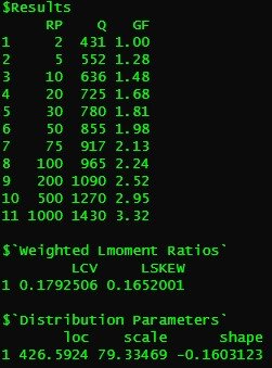
Output from QuickResults function
4. Estimating QMED
There is a QMED function which provides the ungauged QMED estimate and can also provide donor estimates. For the first case it is used as:
QMED(CDs.55002)To undertake a donor transfer, to improve the estimate, a list of donor candidates can be provided. For this there is the DonAdj function, which provides the spatially closest N sites (default of 10) which are suitable for QMED, along with catchment descriptors.
DonAdj(CDs.55002)You can apply a vector of donors using the DonorIDs argument. A vector in ‘R’ is simply a single sample of data, as opposed to a data frame or matrix. To create one, you can use c(datapoint1, datapoint2….datapointN). The following, then, provides a three-donor adjusted QMED:
QMED(CDs.55002, DonorIDs = c(55007, 55016, 55013))Urban donors should be avoided, but donors are “de-urbanised” if they are applied.
Another, quicker, option is to choose the n closest donors by using the no.Donors argument instead of the DonorIDs argument. In both cases you can return the details of the donor catchments using the ReturnDetails argument. For example, if you wanted to apply eight donors and see the associated details of the donors:
QMED(CDs.55002, No.Donors = 8, ReturnDetails = TRUE)In this case the first donor is the subject site so the result will match the observed QMED.
We will save out estimate as an object for use later
MyQMED <- QMED(CDs.55002, No.Donors = 8)5. Creating a pooling group
To create a pooling group, the Pool function can be used. If you specifically want to include or exclude a site, then the include and exclude arguments can be applied.
Pool.55002 <- Pool(CDs = CDs.55002)Pool.55002You may now wish to assess the group for heterogeneity and see which distribution fits best. The H2 function can check for heterogeneity.
H2(Pool.55002)It seems that this site is homogenous. Either way, may wish to use the DiagPlots function to check for any outliers etc. You can also compare with the discordancy measure which can be seen in the second to last column of the pooling group created.
DiagPlots(Pool.55002)Let’s pretend that site 8010 and site 76017 are to be removed. We will also pretend a thorough analysis was undertaken which justified their removal (and the inclusion of any replacements). To remove the sites, we recreate the pooling group and use the exclude option. The function automatically adds the next site/s with the lowest similarity distance measure if the total number of AMAX in the group has dropped below 800 (or whatever we set as the N argument when using the Pool function, which has a default of 800).
Pool.55002 <- Pool(CDs = CDs.55002, exclude = c(8010, 76017))Using the H2 function again the heterogeneity appears to have reduced. We will leave it at that for now and check for the best distribution.
There are two functions to do this and they both compare four distributions; the GEV, the Generalised logistic, the Gumbel, and the Kappa3 distributions. The first is the Zdist outlined in Hosking and Wallis (1997).
Zdists(Pool.55002)In this case it is the Gumbel distribution that appears to fit best. The second is the goodness of tail fit function ‘GoFComparePool’. This latter function scales the pooled AMAX and combines into a single sample. Then RMSE values for each distribution is calculated between the observed scaled flow at each rank and the mean of each rank from 500 samples simulated using the distributions.
GoFComparePool(Pool.55002)Whichever RMSE score is the lowest suggests the better fit. Which, in this case, is also the Gumbel distribution.
We now have all the information needed to estimate our peak flows; the QMED, the pooled group, and the choice of statistical distribution
6. Final estimates (the growth curve and results)
To derive the final estimate the PoolEst function is applied to our pooling group. The QMED option is always required for this function because the user may have further information and data than that provided by the NRFA peak flows AMAX data. We will first get a QMED estimate (in this case we will use the data available from NRFA). To get an estimate of the QMED we can either use the GetAM function and look at the data or we can get it more directly from the observed data embedded within the package. The following code provides the latter.
GetQMED(55002)We can use functions within functions so our use of PoolEst can contain the above command as follows.
PoolEst(Pool.55002, dist = "Gumbel", CDs = CDs.55002, QMEDEstimate = GetQMED(55002), Gauged = TRUE)Note that the Gauged = TRUE argument above only impact the calculation of the factorial standard error (FSE) which is a way to quantify the uncertainty. For example, if we divide and multiply the result for a given return period with the associated FSE raised to the power of 1.96 we get the 95% confidence interval for our estimate.

Results output for the pooled estimate for site 55002
The EVPool function can be used to plot a growth curve (which should look like the below).
EVPool(Pool.55002, gauged = TRUE, dist = "Gumbel")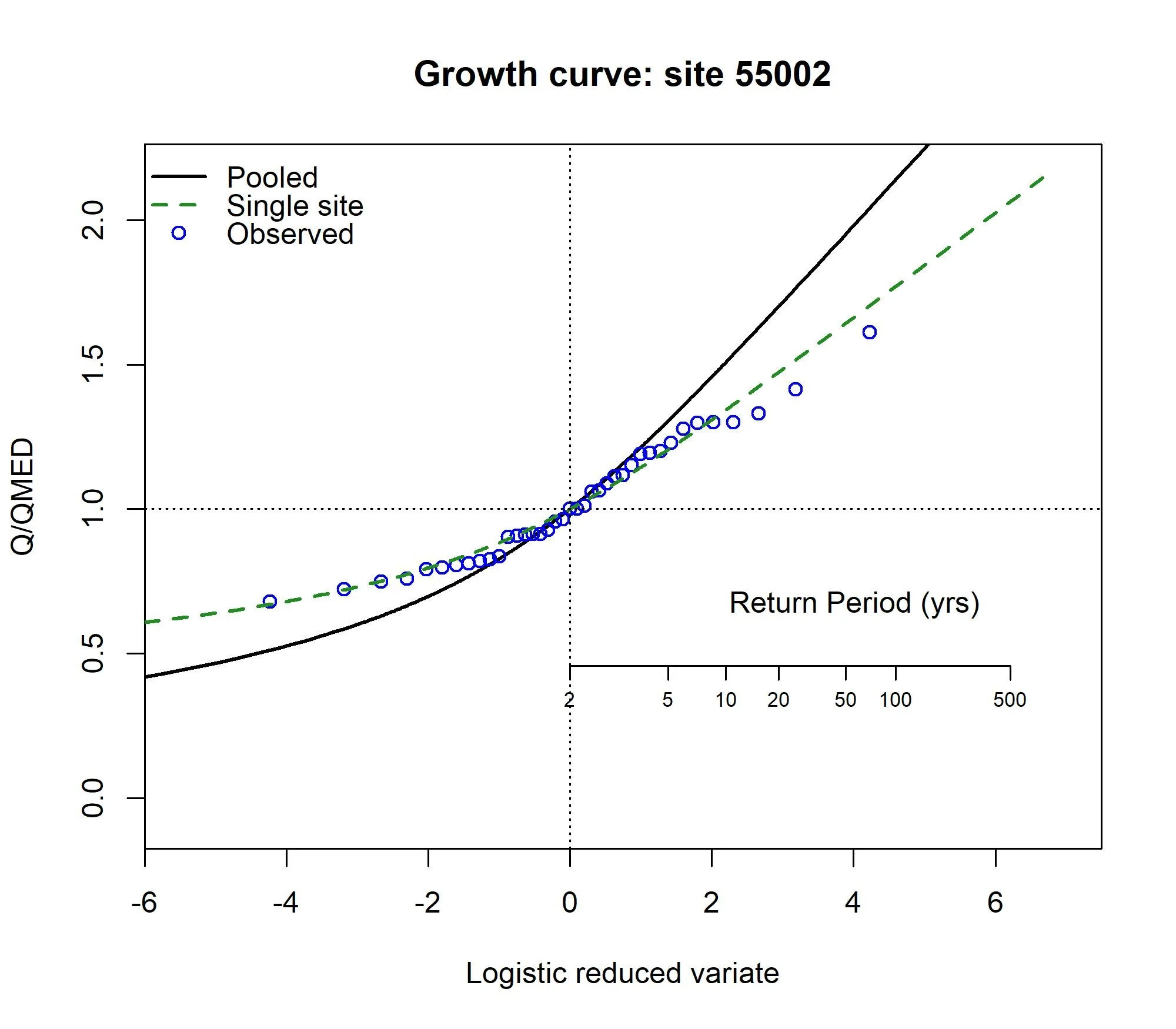
For the ungauged catchment, a similar process can be followed. The calculations are the same but QMED is estimated differently. Here we will use the same descriptors but pretend it is ungauged. First, we’ll exclude the site from our pooling group. We will assume we went through a rigorous pooling group analysis and concluded all was well:
PoolUG.55002 <- Pool(CDs.55002, exclude = 55002)Then estimate QMED from the catchment descriptors with two donors:
CDsQmed.55002 <- QMED(CDs.55002, DonorIDs = c(55007, 55016))Now we’ll use the pooling group and the ungauged QMED estimate to provide the pooled estimates, and then plot the pooled growth curve:
Results55002 <- PoolEst(PoolUG.55002, QMED = CDsQmed.55002, CDs = CDs.55002)and print the results and plot a frequency curve for the pooling group.
Results55002EVPool(PoolUG.55002)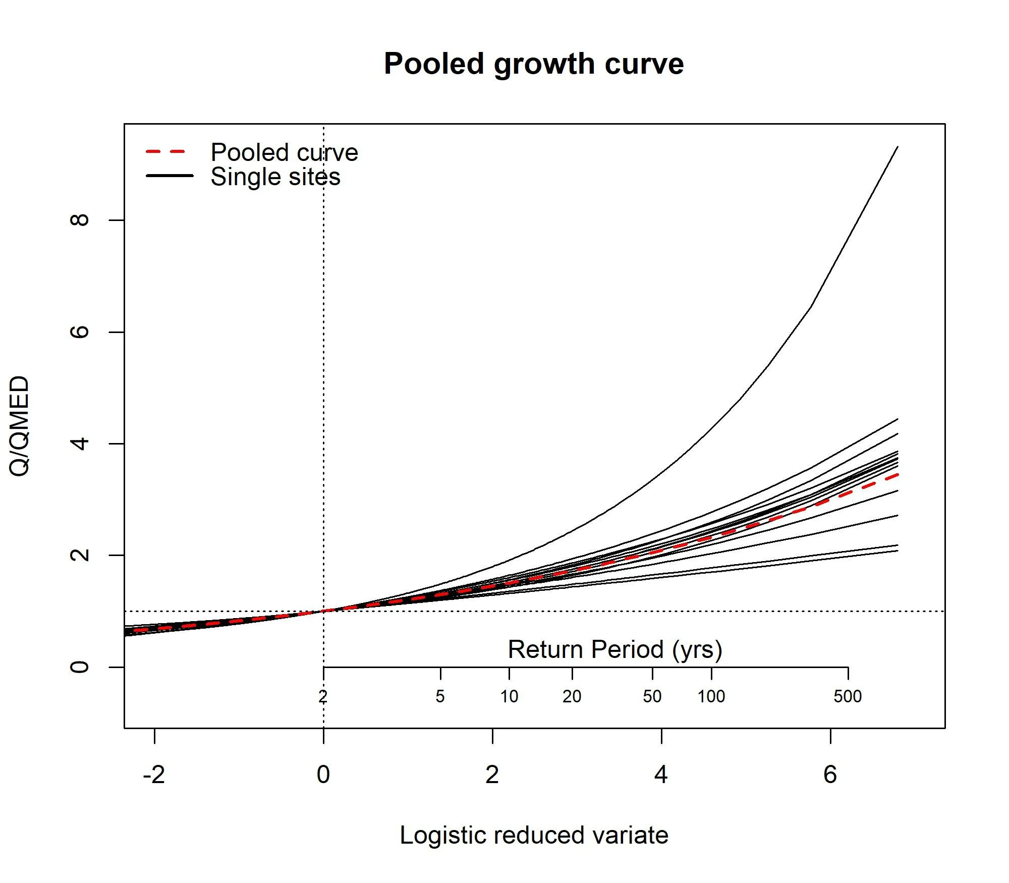
7. Using ReFH and exporting results
The ReFH function is designed for flexibility and each parameter of the model, along with the inputs and initial conditions can be user defined. By default the function provides parameters and settings according to the original ReFH model (ReFH1) as detailed in the 2007 Flood Estimation Handbook supplementary report. However, the function is flexible enough to form other unit hydrograph models. For example, you can change the unit hydrograph to “FSR”, set the BR parameter to zero, and use the Loss argument - which provides a constant proportional loss to the rainfall and the result will then be the FSR/FEH rainfall runoff model. You can also apply an urban loss model (as used in the ReFH2.3 version of the model) or a gamma form for the unit hydrograph.
By default the ReFH1 model is applied with an estimate of RMED as the rainfall depth for the estimated critical duration, with an FSR rainfall profile. However, a rainfall depth can be applied, as can a rainfall vector (some observed rainfall for example). Here is the default output for the catchment we have been looking at.
ReFH(CDs.55002)
Figure 3: Default ReFH output for catchment 55002
We can choose choose a “random” rainfall profile too. As with the FSR rainfall profiles, they’re perhaps not suitable for longer duration, and the example site we’re using (55002 - the Wye at Belmont) has quite a long default duration. Here I have adjusted the time to peak, the duration, the unit hydrograph shape (gamma), and set the rainfall profile to be randomly generated but more inclined to a “central” peak (note that this is not an attempt to better represent the catchment - it is only to demonstrate various options).
RRResults <- ReFH(CDs.55002, TP = 6, Duration = 12, Depth = 20, RainProfile = "Centre", Loss = 0.5, UHShape = "Gamma")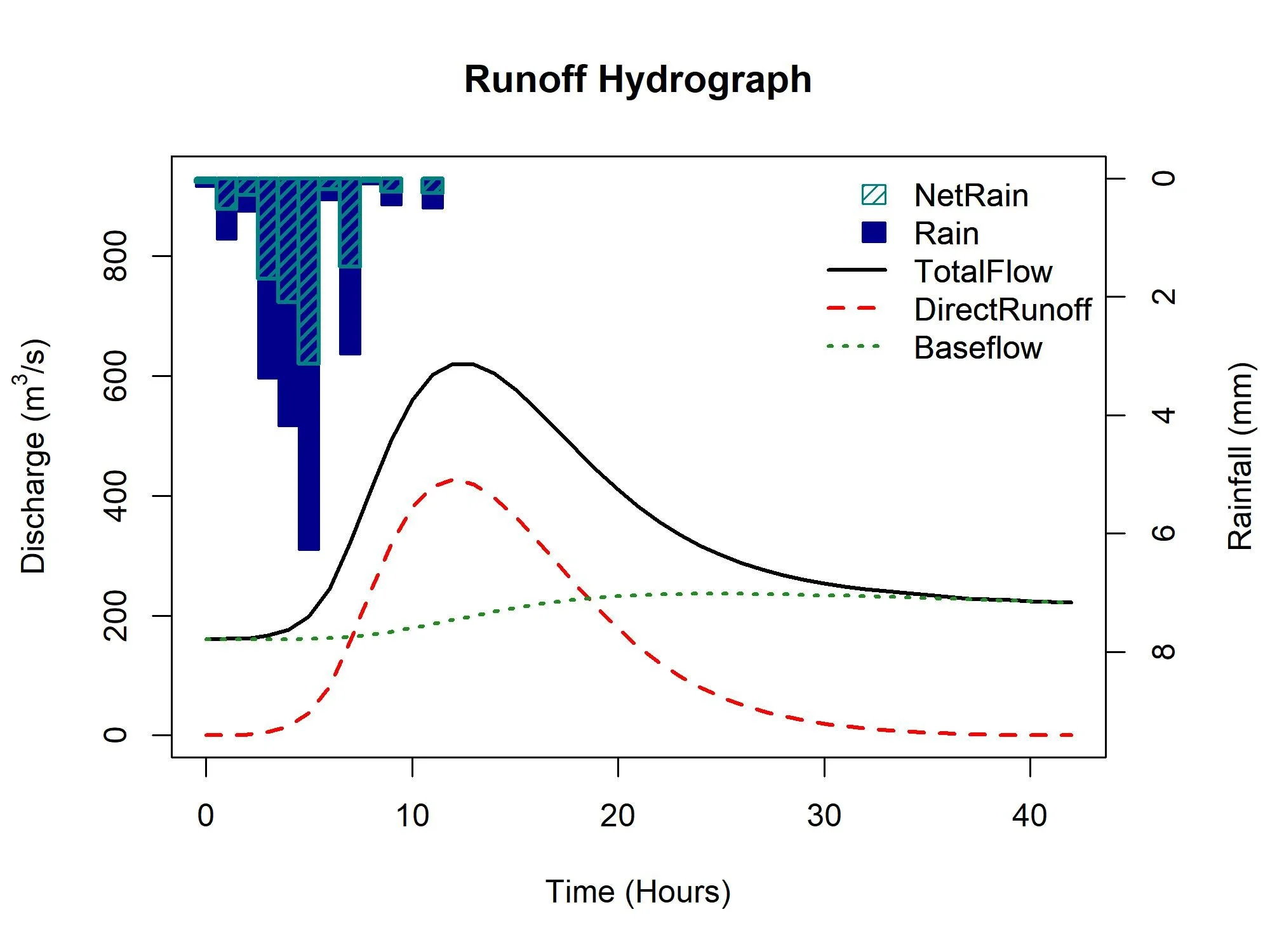
The results are in the form of a list. The first element provides the details of the model, the peak flow and the rainfall depth applied. The second element is a dataframe with the input of rainfall, the net rainfall, the resulting baseflow, runoff and total flow.
RRResultsFor use outside of ‘R’ these outputs can be saved as objects and then written to csv files. Here we save the second element (the results) to a csv file:
write.csv(RRResults[[2]], r"{my/file/path/ReFHResults.csv}", row.names = FALSE)8. Single Site Analysis
The quickest way to get results for a single sample are the GEV, GenLog, Gumbel, Kappa3, and GenPareto functions. For example, for a 75-year return period estimate for an AMAX sample called MyAMAX and using the generalised logistic distribution:
GenLogAM(MyAMAX, RP = 75)An annual maximum series can be obtained for sites suitable for pooling or QMED using the GetAM function. For all other AM series available from the NRFA peaks flows, the AMImport function can be used. If you have a timeseries of flow with associated timestamp, the AnnualStat function can be used to extract the water year AMAX. For now, we will get and plot the AMAX for our site 55002.
AM.55002 <- GetAM(55002)AMplot(AM.55002)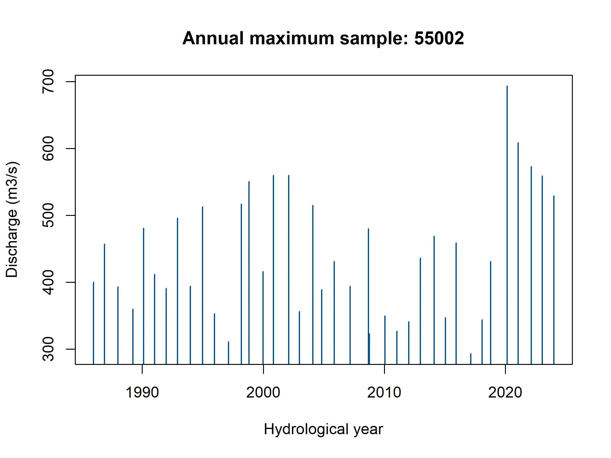
Figure 5: AMAX histogram and bar plot for site 55002
8.1 Annual maximums
For each of the GEV, GenLog, Gumbel, Kappa3, and GenPareto distributions there are four functions; one that estimates return levels or return periods directly from the AM or POT series, one that does the same with an input of parameters, a third that provides the growth factors as a function of Lcv, Lskew and RP, and one for estimating parameters from a AM or POT series.
With our AMAX, we can check the fit of the distributions using the GoFCompare function.
GoFCompare(AM.55002$Flow)It seems the GEV is the better fit for this site. As an example, we can estimate the 100-year flow. Then estimate the RP of the maximum flow observed - during the February 2020 flood (make sure to select the “Flow” column).
GEVAM(AM.55002$Flow, RP = 100)GEVAM(AM.55002$Flow, q = 689)Now estimate the parameters of the GEV from the data, using the default L-moments
GEVPars55002 <- GEVPars(AM.55002$Flow)GEVEst(GEVPars55002[1], GEVPars55002[3] , GEVPars55002[3], RP = 75)If we derive Lmoments for the site, we can then estimate the 50-year growth factor. The Lmoms function does this. We can also calculate LCV and LSKEW separately using the Lcv and LSkew functions. The growth factor can be calculated using the following code
GEVGF(lcv = Lcv(AM.55002$Flow), lskew= LSkew(AM.55002$Flow), RP = 50)Combining this latter result with the median, we can estimate the 50-year flow.
GEVGF(lcv = Lcv(AM.55002$Flow), lskew= LSkew(AM.55002$Flow), RP = 50) * median(AM.55002$Flow)8.2 Peaks over threshold
A POT series can also be obtained from a timeseries using the POTextract function (the POTt function can also be used). There is a daily sample of Thames at Kingston flow within the package that can be used for example purposes. The POTextract function can be used on a single vector or a data frame, with dates in the first column and the timeseries of interest in the second. As the Thames flow is in the third column and the date in the first, for the Thames data the following command can be used.
POT.Thames <- POTextract(ThamesPQ[,c(1,3)], thresh = 0.9)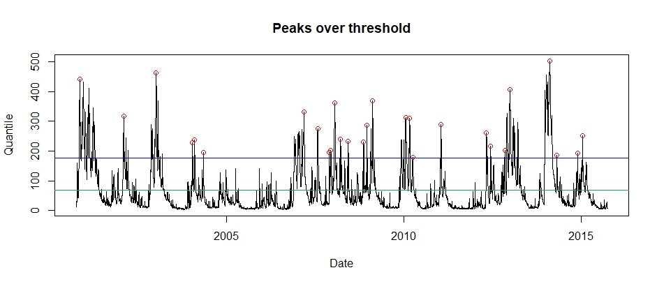
Figure 7: Peaks over threshold for the Thames at Kingson (2000 to 2015). The blue line is the threshold and the green is the mean flow line. Independent peaks are chosen above the threshold. If peaks are separated by a drop below the green line, they are considered independent.
The POT approach is the same except that we need to convert from the POT RP scale to the annual RP scale. To do so, the functions have a peaks per year (ppy) argument. The results of the POTextract function can provide the number of peaks per year (in this case 1.867). To estimate the associated 100-year flow the GenPareto function can be used as follows:
GenParetoPOT(POT.Thames$peak, ppy = 1.867, RP = 100)9. Uncertainty
Uncertainty is quantified as a default when using the PoolEst function. The uncertainty is quantified in the form of the factorial standard error for each estimate. For a single sample of data uncertainty can be quantified for any given statistic using the “Bootstrap” function.
9.1 Single Site
Extract an annual maximum sample with the following code.
AM.55002 <- GetAM(55002)The uncertainty for the 100-year flow can be estimated using the Bootstrap function is then:
Bootstrap(AM.55002$Flow, GEVAM, RP = 100)9.2 Pooling uncertainty
The uncertainty for the pooled estimates is quantified as the factorial standard error (FSE) for each estimate. By default it is estimated as if the subject catchment is ungauged. The FSE for the QMED estimate has a default of 1.5 within the PoolEst function. This can be changed using the fseQMED argument. For example, we may have an observed QMED, but have no confidence in the data for the growth curve estimation. Or we may have a gauged QMED only a kilometre or so upstream, and therefore we might have more confidence for the site of interest and use the observed FSE (which can be determined using the QMEDfseSS function).
If the subject site is gauged and the site is considered suitable for pooling, then the Gauged = TRUE argument can be used in the PoolEst function.
Here is an example> Let’s pretend that our catchment is ungauged and we have a gauge 1km downstream which has an id of 55007. We will then assume we are more confident in our QMED estimate and attribute it an FSE somewhere between the default ungauged FSE and and the observed FSE at 55007.
QMEDEst <- QMED(CDs.55002, DonorIDs = 55007)FSE.MyQMED <- (QMEDfseSS(GetAM(55007)[,2]) + 1.5)/2Now we create the pooling group and estimate QMED with an adjusted FSE for QMED:
PoolUG.55002 <- Pool(CDs.55002, exclude = 55002)PoolEst(PoolUG.55002, QMEDEstimate= QMEDEst, CDs = CDs.55002, fseQMED = FSE.MyQMED)If it were gauged we use Gauged = TRUE as follows:
Pool.55002 <- Pool(CDs.55002)PoolEst(Pool.55002, QMEDEstimate= GetQMED(55002), CDs = CDs.55002, Gauged = TRUE)